CN-Wheat User Guide ¶

Contents

Introduction ¶

CN-Wheat is a Functional-Structural Plant Model which simulates the distribution of carbon and nitrogen into wheat culms in relation to photosynthesis, N uptake, metabolite turnover, root exudation and tissue death. This model can therefore predict the temporal variations and the distribution of carbon and nitrogen into wheat culms.

This model was first produced as part of the project BreedWheat over the last three years, through the Investment for the Future programme managed by the French Research National Agency (ANR-10-BTBR-03). The aim of the project BreedWheat was to improve the competiveness of the French wheat breeding sector, through the definition/ identification of ideotypes, parameters of interest maximizing grain yield and quality under sustainable agricultural systems and climate scenarios.

These researches lead to the publication of project report, and two articles:

Barillot, R., Chambon, C., & Andrieu, B. (2016). CN-Wheat, a functional–structural model of carbon and nitrogen metabolism in wheat culms after anthesis. I. Model description. Annals of Botany, 118(5), 997‑1013. https://doi.org/10.1093/aob/mcw143
and Barillot, R., Chambon, C., & Andrieu, B. (2016). CN-Wheat, a functional–structural model of carbon and nitrogen metabolism in wheat culms after anthesis. II. Model evaluation. Annals of Botany, 118(5), 1015‑1031. https://doi.org/10.1093/aob/mcw144

For installation, testing and deployment: please see file README.md.

Implementation and architecture ¶

Software design ¶

Programming language ¶

CN-Wheat is a software implemented as a Python package, using the Python programming language (http://www.python.org/).

Project tree ¶

The project of CN-Wheat consists of several files and directories:

cnwheat/ is the Python package, i.e. the sources of CN-Wheat (see Package architecture),
test/ is for the unit test,
- test_cnwheat.py: the script to run the unit test,
- input/: the inputs used for the unit test,
- outputs/: the expected and actual outputs of the unit test,
doc/ contains the user and reference (i.e. API) documentations,
- index.rst: the main page of the documentation,
- user.rst: the user guide (this is what you are currently reading…),
- ref.rst: the reference guide (a.k.a. API documentation),
- conf.py: the configuration file used to build the documentation,
- _build/: directories and files generated by library Sphinx when building the documentation,
  
  pickled/: caches of the source “*.rst” documents (not needed to display the HTML documentation),
  
  html/: the HTML documentation generated by Sphinx,
- _static/: custom static files (such as style sheets or script files) generated by library Sphinx,
example/ is a full example which shows how to run a simulation
- main.py: the script used to run the example,
- inputs/: the inputs of CN-Wheat,
- outputs/: the outputs generated by CN-Wheat,
- graphs/: the validation graphs,
- logging.json: the configuration of the logging,
AUTHORS: the authors of CN-Wheat,
LICENCE: the license of CN-Wheat,
README.md: the Read Me file,
setup.cfg: the configuration file used by Setuptools for the deployment of CN-Wheat,
setup.py: the setup script used for the installation of CN-Wheat,
TODO: the todo items.

Package architecture ¶

CN-Wheat is a Python package which consists of several Python modules:

cnwheat: the file to make Python treat directory cnwheat/ as a Python packages,
cnwheat.model: the state and the equations of the model,
cnwheat.parameters: the parameters of the model,
cnwheat.simulation: the simulator (front-end) to run the model,
cnwheat.postprocessing: the post-processing and graph functions,
cnwheat.tools: tools to help for the validation of the outputs,
and cnwheat.converter: functions to convert CN-Wheat inputs/outputs to/from Pandas dataframes.

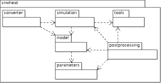
CN-Wheat architecture

Package dependencies ¶

CN-Wheat relies on several Python libraries:

Python (http://www.python.org/), NumPy (http://www.numpy.org/), SciPy (http://www.scipy.org/), Pandas (http://pandas.pydata.org/), Respi-Wheat (https://sourcesup.renater.fr/projects/respi-wheat): implementation and deployment of the model,
Matplotlib (http://matplotlib.org/): generation of graphs to help to validate the model,
Sphinx (http://sphinx-doc.org/): building of the documentation,
Nose (http://nose.readthedocs.org/): run of the automated tests,
and Coverage (http://nedbatchelder.com/code/coverage/): coverage of code testing.

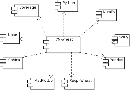
CN-Wheat dependencies

Parameters, variables and equations ¶

CN-Wheat is defined at culm scale, the crop being represented as a population of individual culms. Culms are considered as a set of botanical modules representing the root system, each photosynthetic organ and the whole grains.

Botanical description of the culm structure of wheat as implemented in the model (Barillot et al., 2016)

Computationally, the population is described as a composition of objects, organized in a multiscale tree-like structure:

a population contains one or several plant(s),
- each plant contains one or several axis(es),
  
  each axis contains:
  
  one set of roots,
  
  one phloem,
  
  zero or one set of grains,
  
  and one or several phytomer(s) ; each phytomer contains:
  
  one chaff ; each chaff contains:
  
  one exposed chaff element,
  
  and/or one enclosed chaff element,
  
  and/or one peduncle ; each peduncle contains:
  
  one exposed peduncle element,
  
  and/or one enclosed peduncle element,
  
  and/or one lamina ; each lamina contains:
  
  one exposed lamina element,
  
  and/or one enclosed lamina element,
  
  and/or one internode ; each internode contains:
  
  one exposed internode element,
  
  and/or one enclosed internode element,
  
  and/or one sheath ; each sheath contains:
  
  one exposed sheath element,
  
  and/or one enclosed sheath element.

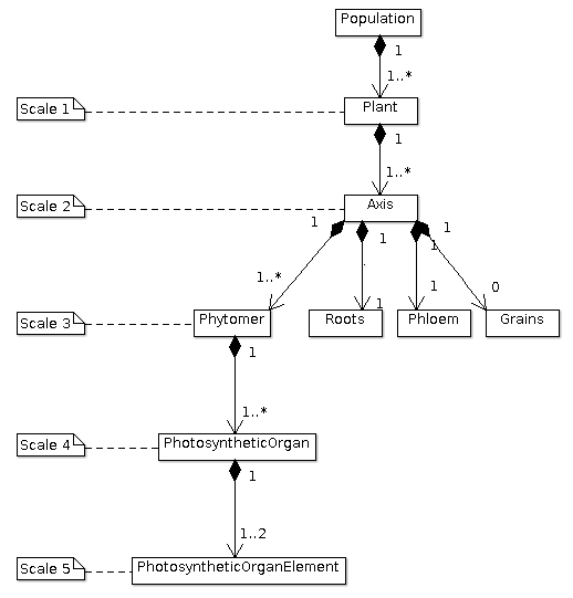
The multiscale tree-like structure of a population of plants

The nitrate concentration in soil is stored and computed in objects of type cnwheat.model.Soil.

These objects include structural, storage and mobile materials, variations in which are represented by ordinary differential equations driven by the main metabolic activities. Each object consists of different metabolites and is connected to a common pool, the phloem, to allow C–N fluxes.

Thus, each class of cnwheat.model defines:

constants to represent the parameters of the model,
attributes to store the current state of the model as compartment values,
and methods to compute fluxes and derivatives in the system of differential equations.

The parameters of the model are stored in module parameters. Module parameters follows the same tree-like structure as module model.

Front-end ¶

Module simulation is the front-end of CN-Wheat. It permits to initialize and run a simulation.

At initialization step, we first check the consistency of the population and soils given by the user. Then we set the initial conditions which will be used by the solver.

When we run the model over 1 time step, we first update the initial conditions. Then we call the function odeint of the library SciPy to integrate the system of differential equations over 1 time step. The derivatives needed by odeint are computed by method _calculate_all_derivatives. If no error occurs and odeint manages to integrate the system successfully, then we update the state of the model setting the attributes of population and soils to the compartment values returned by odeint, and we compute the integrative variables of the population.

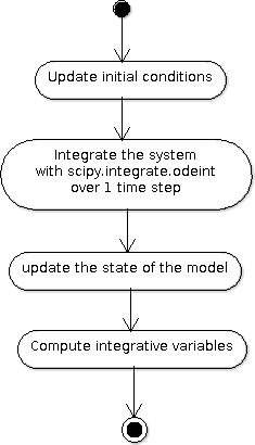
A run of the model

Module simulation also implements exception handling logging, and a progress-bar.

Postprocessing, graphs and tools ¶

After running the simulation over 1 or several time steps, the user can apply postprocessing on the outputs of the model. These post-processing are defined in module postprocessing, and can be computed using function postprocessing.postprocessing.

Module postprocessing also provides a front-end to automate the generation of graphs. These graphs are useful for the validation of the model.

Finally, module tools defines functions to:

plot multiple variables on the same graph,
set up loggers,
check the outputs of the model quantitatively,
and display a progress-bar.

Module converter implements functions to convert CN-Wheat internal population and soils to and from Pandas dataframes.

Constraints on use ¶

Consistency of the inputs ¶

The input population given by the user must the following topological rules:

the population contains at least one plant,
each plant contains at least one axis,
each axis must have:
- one set of roots,
- one phloem,
- zero or one set of grains,
- at least one phytomer,
each phytomer must have at least:
- one photosynthetic organ, among chaff, peduncle, lamina, internode, or sheath,
- or one hiddenzone,
each photosynthetic organ must have one enclosed element and/or one exposed element. Elements enclosed and exposed must be of a type derived from class PhotosyntheticOrganElement, that is one of chaff element, lamina element, internode element, peduncle element or sheath element. An element must belong to an organ of the same type (e.g. a lamina element must belong to a lamina).

Likewise, the input soils given by the user must supply a soil for each axis.

These rules prevent from inconsistency in the modeled system. There are checked automatically at initialization step. If the population or the soils breaks these rules, then the simulator raises an exception with appropriate error message.

Continuity of the model ¶

To integrate the system of ordinary differential equations (ODE), the function odeint takes as first parameters a function which computes the derivatives at t0:

dy/dt = func(y, t0, ...)

where y is a vector.

This function is also called RHS (Right Hand Side) function.

In CN-Wheat, the RHS function is defined by the method _calculate_all_derivatives.

If the RHS function has a discontinuity, this may lead to integration failure, the raise of an exception, and a premature end of the execution. A discontinuity in RHS function could be due to the use of inconsistent parameters or to bug(s) in the equations of the model.

If you get a warning of type “ODEintWarning: Excess work done on this call (perhaps wrong Dfun type)”, you can try to increase the value of ODEINT_MXSTEP defined in the body of the method run. But you should first enable and check the logs to see if you can settle the problem ahead of the integration. Sometimes, this warning is just due to a local discontinuity which does not affect the whole result of the simulation.

Execution time ¶

With an Intel® Core™ i7-5600U CPU @ 2.60GHz × 4 and 7,7 Gio RAM, the simulation example runs in 13.82 s. This example corresponds to a population of one plant with one axis and four phytomers.

Running an example ¶

In one word ¶

To run an example of simulation:

open a command line interpreter,
go to the directory example/ of your local copy of project CN-Wheat,
run command: python main.py.

By default, this example also computes post-processing and generates graphs for validation. You can change this by changing the values of the arguments of the function main.

Here is an activity diagram of this example:

Dataflow of the example

Step by step ¶

Here we explain the simulation example, step by step. The sources of this example and the needed data and configuration files can all be found in the directory example/ of CN-Wheat. So to run the following commands, you need first to go to the directory example/ and open an interpreter IPython.

This example simulates the carbon and nitrogen distribution in a population consisting of:

1 plant,
1 axis,
4 metamers,
1 leaf and 1 stem elements on metamers 1, 2 and 3,
and 1 leaf element on metamer 4.

We use photosynthesis and senescence data computed from others specific models, and made available for CN-Wheat as CSV files.

The simulation runs on a 48 hours time grid, with a constant time step of 4 hours. Photosynthesis and senescence data are forced at each time step.

Inputs are read from CSV files in directory example/inputs/, and outputs are written to CSV files in directory example/outputs/. See Inputs and outputs for more information about the inputs and outputs of the model.

This example also computes post-processing and generates graphs. Post-processing and graphs are saved respectively as CSV and PNG files, in directories example/postprocessing/ and example/graphs/.

Step 1: run the simulation ¶

We first import the packages used by the example, and we define some aliases:

import os
import logging

import pandas as pd

from respiwheat import model as respiwheat_model
from cnwheat import simulation as cnwheat_simulation, converter as cnwheat_converter, \
    tools as cnwheat_tools, postprocessing as cnwheat_postprocessing

Then, we define where the paths of the inputs, the outputs, the post-processing and the graphs:

# inputs directory path
INPUTS_DIRPATH = 'inputs'

# the file names of the inputs
ORGANS_INPUTS_FILENAME = 'organs_inputs.csv'
HIDDENZONES_INPUTS_FILENAME = 'hiddenzones_inputs.csv'
ELEMENTS_INPUTS_FILENAME = 'elements_inputs.csv'
SOILS_INPUTS_FILENAME = 'soils_inputs.csv'

# the file names of the data used to force photosynthesis and senescence parameters
PHOTOSYNTHESIS_ELEMENTS_DATA_FILENAME = 'photosynthesis_elements_data.csv'
SENESCENCE_ROOTS_DATA_FILENAME = 'senescence_roots_data.csv'
SENESCENCE_ELEMENTS_DATA_FILENAME = 'senescence_elements_data.csv'

# outputs directory path
OUTPUTS_DIRPATH = 'outputs'

# CSV file paths to save the outputs of the model in
AXES_OUTPUTS_FILENAME = 'axes_outputs.csv'
ORGANS_OUTPUTS_FILENAME = 'organs_outputs.csv'
HIDDENZONES_OUTPUTS_FILENAME = 'hiddenzones_outputs.csv'
ELEMENTS_OUTPUTS_FILENAME = 'elements_outputs.csv'
SOILS_OUTPUTS_FILENAME = 'soils_outputs.csv'

# post-processing directory path
POSTPROCESSING_DIRPATH = 'postprocessing'

# CSV file paths to save the post-processing of the model in
AXES_POSTPROCESSING_FILENAME = 'axes_postprocessing.csv'
ORGANS_POSTPROCESSING_FILENAME = 'organs_postprocessing.csv'
HIDDENZONES_POSTPROCESSING_FILENAME = 'hiddenzones_postprocessing.csv'
ELEMENTS_POSTPROCESSING_FILENAME = 'elements_postprocessing.csv'
SOILS_POSTPROCESSING_FILENAME = 'soils_postprocessing.csv'

# the path of the directory to save the generated graphs in
GRAPHS_DIRPATH = 'graphs'

We then need to define culm density (in culm.m-2):

CULM_DENSITY = {1:410}

the precision of floats used to write and format outputs and post-processing CSV files:

OUTPUTS_PRECISION = 6

and the number of seconds in 1 hour:

HOUR_TO_SECOND_CONVERSION_FACTOR = 3600

For the logging, we define the path of the configuration file and the logging level:

# config file path for logging
LOGGING_CONFIG_FILEPATH = 'logging.json'

# logging level
LOGGING_LEVEL = logging.INFO # can be one of: DEBUG, INFO, WARNING, ERROR or CRITICAL

To increase the level of logging: set it to logging.DEBUG. To decrease it: setting it to either logging.WARNING, logging.ERROR or logging.CRITICAL. See documentation of module logging for more information.

To force the senescence and photosynthesis data of the population at step of the simulation, we define a function force_senescence_and_photosynthesis():

def force_senescence_and_photosynthesis(t, population, senescence_roots_data_grouped, senescence_elements_data_grouped, photosynthesis_elements_data_grouped):
    '''Force the senescence and photosynthesis data of the population at `t` from input grouped dataframes'''
    for plant in population.plants:
        for axis in plant.axes:
            # Root growth and senescence
            group = senescence_roots_data_grouped.get_group((t, plant.index, axis.label))
            senescence_data_to_use = group.loc[group.first_valid_index(), cnwheat_simulation.Simulation.ORGANS_STATE].dropna().to_dict()
            axis.roots.__dict__.update(senescence_data_to_use)
            for phytomer in axis.phytomers:
                for organ in (phytomer.chaff, phytomer.peduncle, phytomer.lamina, phytomer.internode, phytomer.sheath):
                    if organ is None:
                        continue
                    for element in (organ.exposed_element, organ.enclosed_element):
                        if element is None:
                            continue
                        # Element senescence
                        group_senesc = senescence_elements_data_grouped.get_group((t, plant.index, axis.label, phytomer.index, organ.label, element.label))
                        senescence_data_to_use = group_senesc.loc[group_senesc.first_valid_index(), cnwheat_simulation.Simulation.ELEMENTS_STATE].dropna().to_dict()
                        element.__dict__.update(senescence_data_to_use)
                        # Element photosynthesis
                        group_photo = photosynthesis_elements_data_grouped.get_group((t, plant.index, axis.label, phytomer.index, organ.label, element.label))
                        photosynthesis_elements_data_to_use = group_photo.loc[group_photo.first_valid_index(), cnwheat_simulation.Simulation.ELEMENTS_STATE].dropna().to_dict()
                        element.__dict__.update(photosynthesis_elements_data_to_use)

When called, function force_senescence_and_photosynthesis() updates the parameters and variables of the population which are associated to the senescence and photosynthesis of the modelized population of plants. To do so, force_senescence_and_photosynthesis() takes as arguments grouped Pandas dataframes describing the senescence and photosynthesis per topological scale: roots or elements of organs.

To run a simulation, we first set up the logging:

cnwheat_tools.setup_logging(config_filepath=LOGGING_CONFIG_FILEPATH, level=LOGGING_LEVEL,
                            log_model=False, log_compartments=False, log_derivatives=False)

Log are now written according to the logging configuration file located at path LOGGING_CONFIG_FILEPATH.

Then, we create the simulation, we read inputs from Pandas dataframes, we convert inputs to a population of plants and a dictionary of soils, and we initialize the simulation from the population and the soils:

# create the simulation
simulation_ = cnwheat_simulation.Simulation(respiration_model=respiwheat_model, delta_t=3600, culm_density=CULM_DENSITY)

# read inputs from Pandas dataframes
inputs_dataframes = {}
for inputs_filename in (ORGANS_INPUTS_FILENAME, HIDDENZONES_INPUTS_FILENAME, ELEMENTS_INPUTS_FILENAME, SOILS_INPUTS_FILENAME):
    inputs_dataframes[inputs_filename] = pd.read_csv(os.path.join(INPUTS_DIRPATH, inputs_filename))

# convert inputs to a population of plants and a dictionary of soils
population, soils = cnwheat_converter.from_dataframes(inputs_dataframes[ORGANS_INPUTS_FILENAME],
                                                      inputs_dataframes[HIDDENZONES_INPUTS_FILENAME],
                                                      inputs_dataframes[ELEMENTS_INPUTS_FILENAME],
                                                      inputs_dataframes[SOILS_INPUTS_FILENAME])

# initialize the simulation from the population and the soils
simulation_.initialize(population, soils)

Then, we get photosynthesis and senescence data from CSV files, we group them, we create empty lists of dataframes to store the outputs at each step, and we define the time grid to run the model on:

# get photosynthesis data
photosynthesis_elements_data_filepath = os.path.join(INPUTS_DIRPATH, PHOTOSYNTHESIS_ELEMENTS_DATA_FILENAME)
photosynthesis_elements_data_df = pd.read_csv(photosynthesis_elements_data_filepath)
photosynthesis_elements_data_grouped = photosynthesis_elements_data_df.groupby(cnwheat_simulation.Simulation.ELEMENTS_T_INDEXES)

# get senescence and growth data
senescence_roots_data_filepath = os.path.join(INPUTS_DIRPATH, SENESCENCE_ROOTS_DATA_FILENAME)
senescence_roots_data_df = pd.read_csv(senescence_roots_data_filepath)
senescence_roots_data_grouped = senescence_roots_data_df.groupby(cnwheat_simulation.Simulation.AXES_T_INDEXES)
senescence_elements_data_filepath = os.path.join(INPUTS_DIRPATH, SENESCENCE_ELEMENTS_DATA_FILENAME)
senescence_elements_data_df = pd.read_csv(senescence_elements_data_filepath)
senescence_elements_data_grouped = senescence_elements_data_df.groupby(cnwheat_simulation.Simulation.ELEMENTS_T_INDEXES)

# create empty lists of dataframes to store the outputs at each step
axes_outputs_df_list = []
organs_outputs_df_list = []
hiddenzones_outputs_df_list = []
elements_outputs_df_list = []
soils_outputs_df_list = []

# define the time grid to run the model on
start_time = 0
stop_time = 48
time_step = 4
time_grid = xrange(start_time, stop_time+time_step, time_step)

Then, we force the senescence and photosynthesis of the population by calling function force_senescence_and_photosynthesis(), and we reinitialize the simulation from forced population:

# force the senescence and photosynthesis of the population
force_senescence_and_photosynthesis(0, population, senescence_roots_data_grouped, senescence_elements_data_grouped, photosynthesis_elements_data_grouped)

# reinitialize the simulation from forced population
simulation_.initialize(population, soils)

Next, we create the time loop to run a simulation at each step of the time grid. The first step of the time loop is the initial step. We needn’t to run the model for this step. Thus, we just: * convert model outputs to dataframes, * and append the outputs at current t to the global lists of dataframes.

For all others steps t until t >= stop_time, we:

run the model of CN exchanges,
convert model outputs to dataframes,
append the outputs at current t to the lists of dataframes,
force the senescence and photosynthesis of the population,
and reinitialize the simulation from forced population and soils.

Here is the time loop with some comments in the code:

for t in time_grid:

    if t > 0:
        # run the model of CN exchanges ; the population is internally updated by the model
        simulation_.run()

    # convert model outputs to dataframes
    _, axes_outputs_df, _, organs_outputs_df, hiddenzones_outputs_df, elements_outputs_df, soils_outputs_df = cnwheat_converter.to_dataframes(simulation_.population, simulation_.soils)

    # append the outputs at current t to the lists of dataframes
    for df, list_ in ((axes_outputs_df, axes_outputs_df_list), (organs_outputs_df, organs_outputs_df_list),
                      (hiddenzones_outputs_df, hiddenzones_outputs_df_list), (elements_outputs_df, elements_outputs_df_list),
                      (soils_outputs_df, soils_outputs_df_list)):
        df.insert(0, 't', t)
        list_.append(df)

    if t > 0 and t < stop_time:

        # force the senescence and photosynthesis of the population
        force_senescence_and_photosynthesis(t, population, senescence_roots_data_grouped, senescence_elements_data_grouped, photosynthesis_elements_data_grouped)
        # reinitialize the simulation from forced population and soils
        simulation_.initialize(population, soils)

Finally, we write the outputs of the model to CSV files:

outputs_df_dict = {}
for outputs_df_list, outputs_filename in ((axes_outputs_df_list, AXES_OUTPUTS_FILENAME),
                                          (organs_outputs_df_list, ORGANS_OUTPUTS_FILENAME),
                                          (hiddenzones_outputs_df_list, HIDDENZONES_OUTPUTS_FILENAME),
                                          (elements_outputs_df_list, ELEMENTS_OUTPUTS_FILENAME),
                                          (soils_outputs_df_list, SOILS_OUTPUTS_FILENAME)):
    outputs_filepath = os.path.join(OUTPUTS_DIRPATH, outputs_filename)
    outputs_df = pd.concat(outputs_df_list, ignore_index=True)
    outputs_df.to_csv(outputs_filepath, na_rep='NA', index=False, float_format='%.{}f'.format(OUTPUTS_PRECISION))
    outputs_file_basename = outputs_filename.split('.')[0]
    outputs_df_dict[outputs_file_basename] = outputs_df

You should now see the ouputs CSV files in directory OUTPUTS_DIRPATH.

See Inputs and outputs for more information about the outputs of the model.

Step 2: compute the post-processing ¶

To run the post-processing, we first define the base name of each post-processing file:

axes_postprocessing_file_basename = AXES_POSTPROCESSING_FILENAME.split('.')[0]
hiddenzones_postprocessing_file_basename = HIDDENZONES_POSTPROCESSING_FILENAME.split('.')[0]
organs_postprocessing_file_basename = ORGANS_POSTPROCESSING_FILENAME.split('.')[0]
elements_postprocessing_file_basename = ELEMENTS_POSTPROCESSING_FILENAME.split('.')[0]
soils_postprocessing_file_basename = SOILS_POSTPROCESSING_FILENAME.split('.')[0]

Then we call function cnwheat_postprocessing.postprocessing(), passing it the computed outputs as arguments:

delta_t = simulation_.delta_t

postprocessing_df_dict = {}

(postprocessing_df_dict[axes_postprocessing_file_basename],
 postprocessing_df_dict[hiddenzones_postprocessing_file_basename],
 postprocessing_df_dict[organs_postprocessing_file_basename],
 postprocessing_df_dict[elements_postprocessing_file_basename],
 postprocessing_df_dict[soils_postprocessing_file_basename]) \
    = cnwheat_postprocessing.postprocessing(axes_df=outputs_df_dict[AXES_OUTPUTS_FILENAME.split('.')[0]],
                                              hiddenzones_df=outputs_df_dict[HIDDENZONES_OUTPUTS_FILENAME.split('.')[0]],
                                              organs_df=outputs_df_dict[ORGANS_OUTPUTS_FILENAME.split('.')[0]],
                                              elements_df=outputs_df_dict[ELEMENTS_OUTPUTS_FILENAME.split('.')[0]],
                                              soils_df=outputs_df_dict[SOILS_OUTPUTS_FILENAME.split('.')[0]],
                                              delta_t=delta_t)

And we write the post-processing to CSV files:

for postprocessing_file_basename, postprocessing_filename in ((axes_postprocessing_file_basename, AXES_POSTPROCESSING_FILENAME),
                                                                (hiddenzones_postprocessing_file_basename, HIDDENZONES_POSTPROCESSING_FILENAME),
                                                                (organs_postprocessing_file_basename, ORGANS_POSTPROCESSING_FILENAME),
                                                                (elements_postprocessing_file_basename, ELEMENTS_POSTPROCESSING_FILENAME),
                                                                (soils_postprocessing_file_basename, SOILS_POSTPROCESSING_FILENAME)):

    postprocessing_filepath = os.path.join(POSTPROCESSING_DIRPATH, postprocessing_filename)
    postprocessing_df_dict[postprocessing_file_basename].to_csv(postprocessing_filepath, na_rep='NA', index=False, float_format='%.{}f'.format(OUTPUTS_PRECISION))

You should now see the generated post-processing CSV files in directory POSTPROCESSING_DIRPATH.

See Post-processing for more information about the post-processing which can be applied on the outputs of the model.

Step 3: generate the graphs for validation ¶

Finally, to generate the graphs, we simply call function cnwheat_postprocessing.generate_graphs(), with the computed post-processing dataframes as arguments:

cnwheat_postprocessing.generate_graphs(hiddenzones_df=postprocessing_df_dict[HIDDENZONES_POSTPROCESSING_FILENAME.split('.')[0]],
                                       organs_df=postprocessing_df_dict[ORGANS_POSTPROCESSING_FILENAME.split('.')[0]],
                                       elements_df=postprocessing_df_dict[ELEMENTS_POSTPROCESSING_FILENAME.split('.')[0]],
                                       soils_df=postprocessing_df_dict[SOILS_POSTPROCESSING_FILENAME.split('.')[0]],
                                       graphs_dirpath=GRAPHS_DIRPATH)

Script example/main.py put all these codes together, and permits to run either the simulation, the post-processing or the graph generation, or all of them one after the other.

Inputs and outputs ¶

The inputs and the outputs of the model consist in state parameters and state variables describing the state of the population at a given step.

All state parameters and state variables are defined in the classes of the module cnwheat.model. At a given step, instances of these classes stored the state parameters and state variables which represent the state of the system.

See module cnwheat.model for a documentation on the inputs and outputs of the model.

Post-processing ¶

The functions which compute the post-processing are defined in the module cnwheat.postprocessing, by botanical object.

See module cnwheat.postprocessing for a documentation on the post-processing which can be applied on the outputs of the of the model.